DEFINITION OF SUPPLY

Supply is the quantity of goods/services per unit of time which suppliers/producers are willing

and able to put on the market for sale at alternative prices other things held constant.

Individual  Versus Market Supply Curve

(i) Firm and industry supply schedules

The plan or table of possible quantities that will be offered for sale at different prices by

individual firms for a commodity is called supply schedule.

Price Per Unit Quantity offered for

                        (KShs)                                      Sales per month (in ‘000)

                              20                                                       10

                              25                                                       20

                              30                                                       30

                              35                                                       40

                              40                                                       50

                              45                                                       60

                              50                                                       70

The Firm Supply Schedule

Theoretically the supply schedules of all firms within the industry can be combined to form the

market or industry supply schedule, representing the total supply for that commodity at various

prices.

     Price per unit                                       Quantity offered for

         (KShs)                                            Sales per month (in ‘000)

               20                                                            80

               25                                                           120

               30                                                           160

               35                                                           200

               40                                                           240

               45                                                           285

               50                                                           320

Table: The Industry supply schedule

These prices are called the supply prices.

(ii) Individual firm and market supply curves

The quantities and prices in the supply schedule can be plotted on a graph. Such a graph is called

the firm supply curve.

A firm supply curve is a graph relating the price and the quantities of a commodity a firm

is prepared to supply at those prices.

The typical supply curve slopes upwards from left to right. This illustrates the second law of

supply and demand �which states that the higher the price the greater the quantity that will be

supplied�.

More is supplied by the firms which could not make a profit at the lower price

.

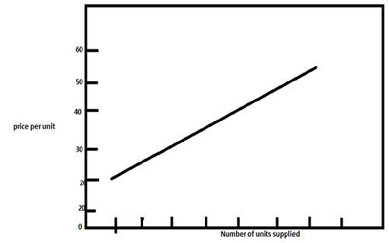
Fig 2. The firm supply curve

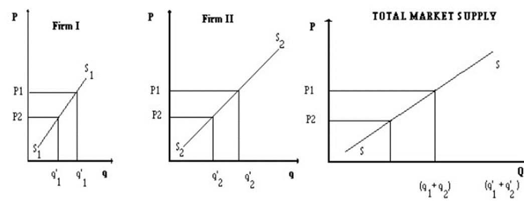
The market supply curve is obtained by horizontal summation of the individual firm supply

curves i.e. taking the sum of the quantities supplied by the different firms at each price.

Consider, for the sake of exposition, an industry consisting of two firms. At price P1, firm I

(diagram below) supplies quantity q1, firm II supplies quantity q2, and the total market supply is

q1+q2

At price P2, firm I supplies q’1, firm II supplies quantity q’2, and the total market supply is q’1+q’2,. SS is the total market supply curve. 

FACTORS INFLUENCING SUPPLY

a) Own Price of the commodity

There is a direct relationship between quantity supplied and the price so that the higher the price,

the more people shall bring forth to the market. Mathematically this can be illustrated as follows:

Qs = -c + dp

Where: Qs is the quantity supplied

-c is a constant

d is the factor by which price changes

P is the price

Thus the normal supply curve slopes upwards from left to right as follows:

organisations which could not produce profitably at the lower price would find it possible to do

so at a higher price. One way of looking at his is that as price goes up, less and less efficient

firms are brought into the industry.

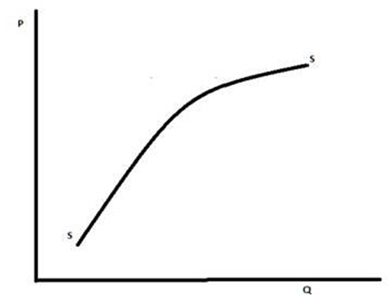
Exceptional supply curves

In have some situations the slope of the supply curve may be reversed.

i) Regressive Supply. In this case, the higher the price within a certain range, the smaller the

amount offered to the market. This may occur for example in some labour markets where above

certain level, higher wages have a disincentive effect as the leisure preference becomes high.

This may also occur in undeveloped peasant economies where producers have a static view of

the income they receive. Lastly regressive supply curves may occur with target workers.

ii) Fixed Supply. Where the commodity is rare e.g. the �Mona Lisa�, the supply remains the

same regardless of price. This will be true in the short term of the supply of all things,

particularly raw materials and agricultural products, since time must elapse before it is physically

possible to increase output.

b) Prices of other related goods

i) Substitutes: If X and Y are substitutes, then if the price X increases, the quantity demanded of

X falls. This will lead to increased demand for Y, and this way eventually lead to increased

supply of Y.

ii) Complements: If two commodities, say A and B are used jointly, then an increase in the price

of A shall lead to a fall in the demand for A, which will cause the demand for B to fall too.

c) Prices of the factors of production

As the prices of those factors of production used intensively by X producers rise, so do the firms�

costs. This cause supply to fall as some firms reduce output and other, less efficient firms make

losses and eventually leave the industry. Similarly, if the price of one factor of production would

rise (say, land), some firms may be tempted to move out of the production of land intensive

products, like wheat, into the production of a good which is intensive in some other factor of

production.

d) Goals of the firm

How much is produced by a firm depends on its objectives. A firm which aims to maximise its

sales revenue, for example, will generally supply a greater quantity than a firm aiming to

maximise profits (see markets). Changes in these objectives will usually lead to changes in the

quantity supplied.

e) State of technology

There is a direct relationship between supply and technology. Improved technology results in

more supply as with technology there is mechanisation.

f) Natural events

Natural events like weather, pests, floods, etc also affect supply. These affect particularly the

supply of agricultural products. If weather conditions are favourable, the supply of agricultural

products will increase. Conversely, if weather conditions are unfavourable the supply of such

products will fall.

g) Time

In the long run (with time), the supply of most products will increase with capital accumulation,

technical progress and population growth so long as the last one takes place in step with the first

two. This reflects economic growth.

h) Supply of Inputs

Changes in supply of inputs will affect the quantity supplied; if this falls, less shall be supplied

and vice versa.

i) Changes in the supply of the product with which the product in question is in joint

supply e.g. hides and skins.

j) Taxes and subsidies

The imposition of a tax on a commodity by the government is equivalent to increasing the costs

of production to the producer because the tax �eats� into the firm�s profits. Hence taxes tend to

discourage production and hence reduce supply. Conversely, the granting of a subsidy is

equivalent to covering the costs of production. Hence subsidies tend to encourage production and

increase supply.

MOVEMENT ALONG AND SHIFTS OF SUPPLY CURVES

i) Movements along the supply curve:

Movements along the supply curve are brought about by changes in the price of the commodity.

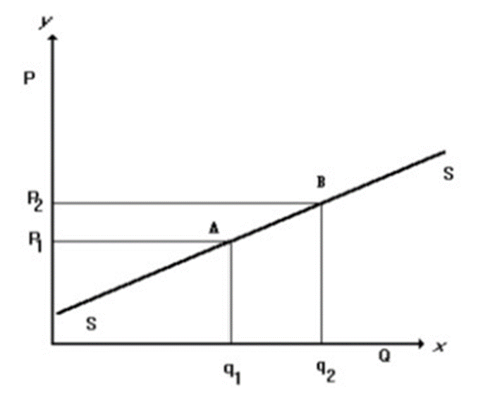
When price increases from P1 to P2, quantity supplied increases from Q1 to Q2 and movement

along the supply curve is from A to B. Conversely when price falls from P2 to P1, quantity

supplied falls from q2 to q1 and movement along the supply curve is from B to A.

ii) Shifts in the supply curve

Shifts in the supply curve are brought about by changes in factors other than the price of the

commodity. A shift in supply is indicated by an entire movement (shift) of the supply curve to

the right (downwards) or to the left (upwards) of the original curve.

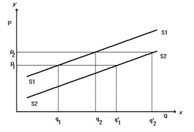
When supply increases, the supply curve shifts to the right from S1S1 to S2S2. At price P1,

supply increases from q1 to q�1 and at price P2 supply increases from q2 to q�2. Conversely, a

fall in supply is indicated by a shift to the left or upwards of the supply curve and less is supplied

at all prices. Thus, when supply falls, the supply curve shifts to the left from position S2S2 to

position S1S1. At price p1, supply falls from q�1 to q1 and at price p2, supply falls from q�2 to q2.

ELASTICITY OF SUPPLY

It refers to the responsiveness of quantity supplied to changes in factors affecting price

PRICE ELASTICITY OF SUPPLY

Definition

Price Elasticity of supply measures the degree of responsiveness of quantity supplied to changes

in price. The co-efficient of the elasticity of supply may be stated as:

Percentage change in quantity supplied

Percentage change in Price

Mathematically, this can be written as:

Symbolically it is given by the formula.

Because of the positive relationship between price and quantity supplied, the price elasticity of supply ranges from zero to infinity. 

TYPES OF ELASTICITY OF SUPPLY

i) Perfectly Inelastic (Zero Elastic) Supply:

Supply is said to be perfectly inelastic if the quantity supplied is constant at all prices. The

supply curve is a vertical straight line and the elasticity of supply is equal to zero.

When price rises from P1 to P2, quantity supplied stays fixed at q, and when price falls from P2

to P1, quantity supplied stays fixed.

In the case of a price rise, this is the situation of the very short-run or the momentary period

which is so short that the quantity supplied cannot be increased, e.g. food brought to the market

in the morning. It is also the case where the commodity is fixed in supply e.g. land. In the case of

a price fall, this is the case of a highly perishable commodity which cannot be stored, e.g. fresh

fish.

ii) Inelastic Supply:

Supply is said to be price inelastic if changes in price bring about changes in quantity supplied in

less proportion. Thus, when price increases quantity supplied increases in less proportion, and

when price falls quantity supplied falls in less proportion. The supply curve is steeply sloped and

the elasticity of supply is less than one.

When price increases from P1 to P2, quantity supplied increases in less proportion from q1 to

q2. This is the case when there are limited stocks of the product or the product takes a long time

to produce such that when price rises, quantity supplied cannot be increased substantially.

Conversely, if price falls from P2 to P1, quantity supplied falls in less proportion from q2 to q1.

This is the case of a commodity which is perishable and cannot be easily stored, e.g. fresh foods

like bananas and tomatoes. These are perishable but not so highly perishable as fresh fish. When

price falls, quantity supplied cannot be drastically reduced.

iii) Unit Elasticity of Supply:

Supply is said to be of unit elasticity if changes in price bring about changes in quantity supplied

in the same proportion. Thus, when price rises, quantity supplied increases in the same

proportion, and when price falls, quantity supplied falls in the same proportion. The supply curve

is a straight line through the origin, and the elasticity of supply is equal to one or unity.

When price rises from P1 to P2, quantity supplied increases in the same proportion from q1 to

q2. This is the case of a commodity of which there is a fair amount of stocks or which can be

produced within a fairly short period of time.

Conversely, when price falls from P2 to P1, quantity supplied falls in the same proportion from

q2 to q1. This is the case of a commodity which is fairly easily stockable, e.g. dry foods, like dry

beans and dry maize.

iv) Elastic Supply

Supply is said to be price elastic if changes in price bring about changes in quantity supplied in

greater proportion. Thus, when price increases, quantity supplied increases in greater proportion.

The supply curve is not steeply sloped and the elasticity of supply is greater than one.

When price rises from P1 to P2, quantity supplied rises in greater proportion from q1 to q2.

This is the case when there are a lot of stocks of the commodity or the commodity can be

produced within fairly short period of time so that when price rises, quantity supplied can be

increased substantially.

Conversely, if price falls from P2 to P1, quantity supplied falls in greater proportion from q2 to

q1. This is the case of a commodity which is easily stockable e.g. manufactured articles.

When price falls, quantity supplied can be substantially reduced. The commodity is then stored

instead of being sold at a loss or for very reduced profit.

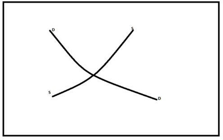
v) Perfectly Elastic Supply

Supply is said to be perfectly or infinitely elastic if the price is fixed at all levels of demand. The

demand curve has been shown in the above diagram for the sake of clarity.

If the supply is perfectly elastic, the supply curve is a horizontal straight line and the elasticity of

supply is equal to infinity.

When demand increases from quantity supplied increases but price stays fixed . Conversely, if

demand falls, quantity supplied falls but price stays fixed.

This is the case of Government price control.

FACTORS INFLUENCING ELASTICITY OF SUPPLY

Time

In the short run firms will only be able to increase input of labor to increase supply of

commodities may not be able to increase the supply in response to the price change but the

supply change will be little because other factors of production may not be increased in the same

proportion and may limit the supply. However, in the long run a firm will increase the input of

all factors of production and thus the supply becomes more price elastic.

Availability of resources

If the economy already using most of its scarce resources then firms will find it difficult to

employ more and so output will not be able to rise. The supply of most of goods and services

will therefore be price inelastic.

Number of producers

More producers mean that the output can be increased more easily. Thus supply is more elastic.

Ease of storing stocks

If goods can be stocked with ease and have a long shelf life, the supply will be elastic, otherwise

inelastic. For example perishable goods such as fresh flowers, vegetables have comparatively

inelastic supply because it is difficult to store them for longer periods.

Increase in cost of production as compared to output

In cases where there is a significant increase in cost of production when output is increased,

supply is inelastic. This is because suppliers will have to have to do a significant investment in

order to increase the output. It will take time and some suppliers may be hesitant in doing so.

Improvement in Technology

In industries where there is a rapid improvement in technology, the PES of such goods will be

more elastic as compared to industries where there is not much improvement in technology.

Stock of finished goods

In industries where there are high inventories/stocks of finished goods, the suppliers can easily

supply more as the price rises. Thus, the PES for these goods will be elastic.

APPLICATION OF ELASTICITY OF SUPPLY

i) If the supply of a commodity is elastic with respect to a price rise, producers will benefit by

prices not rising excessively. But if the supply is inelastic with respect to a price rise, there will

tend to be overpricing of the commodity to the disadvantage of the consumers. Even the

 producers will not benefit as much as they would if the supply was elastic because although they

are charging high prices, the supply is limited.

ii) If the supply is inelastic with respect to a price fall: This increases the risk of the business

because it means that producers may be forced to sell the commodity at very low prices as the

commodity cannot be easily stored. But if the supply is elastic with respect to a price fall, the

business is less risky as the commodity can easily be stored, and producers will not be forced to

sell at low prices.

iii) The price elasticity of supply is responsible for the fact that the prices of agricultural

products tend to fluctuate more than those of manufactured products.

DETERMINATION OF EQUILIBRIUM

Interaction of Supply and Demand, Equilibrium Price and Quantity

In perfectly competitive markets the market price is determined by the interaction of the forces

of demand and supply. In such markets the price adjusts upwards or downwards to achieve a

balance, or equilibrium, between the goods coming in for sale and those being requested by

purchases. Demand and supply react on one another until a position of stable equilibrium is

reached where the quantities of goods demanded equal the quantities of goods supplied. The

price at which goods are changing hands varies with supply and demand. If the supply exceeds

demand at the start of the week, prices will fall. This may discourage some of the suppliers, who

will withdraw from the market, and at the same time it will encourage consumers, who will

increase their demands. This is known as buyers market.

Conversely if we examine line D, where the price is �2 per kg, suppliers are only willing to

supply 90kg per week but consumers are trying to buy 200 kg per week.

There are therefore many disappointed customers, and producers realise that they can raise

prices. This is known as sellers market. There is thus an upward pressure on price and it will rise.

This may encourage some suppliers, who will enter the market, and at the same time it will

discourage consumers, who will decrease their demand.

This can be shown by comparing the demand and supply schedule below.

     Price of Commodity X    Quantity demanded         Quantity supplied             Pressure on

     $/kg                             of commodity X(kg/week)         of commodity X (kg/week)        price 

A Twin force is therefore always at work to achieve only one price where there is neither upward

or downward pressure on price. This is termed the equilibrium or market price:

The equilibrium price is the market condition which once achieved tends to persist or at

which the wishes of buyers and sellers coincide.

Any other price anywhere is called DISEQUILIBRIUM PRICE. As the price falls the quantity

demanded increases, but the quantity offered by suppliers is reduced, since the least efficient

suppliers cannot offer the goods at the lower prices. This illustrates the third "law" of demand

and supply that "Price adjusts to that level which equates demand and supply".

Mathematical  Approach to Equilibrium Analysis

The demand and supply relationships explained earlier on can be expressed in mathematical

form. The standard problem is one of finding a set of values which will satisfy the equilibrium

condition of the market model.

Equilibrium in a single market model.

A single market model has three variables: the quantity demanded of the commodity (Qd), the

quantity supplied of the commodity (Qs) and the price of the commodity (P). equilibrium is

assumed to hold in the market when the quantity demanded (Qd) = Quantity Supplied (Qs) . It is

assumed that both Qd and Qs are functions. A function such as y = f (x) expresses a relationship

between two variables x and y such that for each value of x there exists one and only one value

of y. Qd is assumed to be a decreasing linear function of P which implies that asP increases, Qd decreases and Vice Versa. Qs on the other hand is assumed to be an increasing

linear function of P which implies that as P increases, so does Qs.

Mathematically, this can be expressed as follows:

Qd = Qs

Qd = a – bP where a,b > 0. ................................... (i)

Qs = -c + dp where c,d >0. .................................. (ii)

Both the Qd and Qs functions in this case are linear and can be expressed graphically as follows: Qd, Qs Qd = a - bP QS = -c + dP

Qd = Qs

Once the model has been constructed it can be solved.

At equilibrium,

Qd = Qs

∴a – bP = -c + dP P = a + c b + d

To find the equilibrium quantity Q, we can substitute into either function (i) or (ii). Substituting P into equation (i) we obtain:

Q = a – b (a+c) = a (b+d) – b (a+c) = ad -bc b + d b + d b + d

Taking a numerical example, assume the following demand and supply functions:

P = 100 – 2P

Qs = 40 + 4P

At equilibrium, Qd = Qs

∴ 100 – 2 P = 40 + 4 P

6P = 60

∴ P = 10

Substituting P = 10, in either equation.

Qd = 100 – 2 (10) = 100 – 20 = 80 = Qs 

STABLE VERSUS UNSTABLE EQUILIBRIUM

Enroll Now To Read More